Working with SPH data
First import the Plonk package.
>>> import plonk
We also import Matplotlib and NumPy, for later.
>>> import matplotlib.pyplot as plt
>>> import numpy as np
Snapshots
SPH snapshot files are represented by the Snap class. This object
contains a properties dictionary, particle arrays, which are lazily loaded from
file. Here we demonstrate instantiating a Snap object, and
accessing some properties and particle arrays.
First, we load the snapshot with the load_snap() function. You can
pass a string or pathlib.Path object to point to the location of the
snapshot in the file system.
>>> filename = 'disc_00030.h5'
>>> snap = plonk.load_snap(filename)
You can access arrays by their name passed in as a string.
>>> snap['position']
array([[-3.69505001e+12,  7.42032967e+12, -7.45096980e+11],
       [-1.63052677e+13,  1.16308971e+13,  1.92879212e+12],
       [-7.66283930e+12,  1.62532232e+13,  2.34302988e+11],
       ...,
       [ 1.39571712e+13, -1.16179990e+13,  8.09090354e+11],
       [ 9.53716176e+12,  9.98500386e+12,  4.93933367e+11],
       [ 1.21421196e+12,  2.08618956e+13,  1.12998892e+12]]) <Unit('meter')>
There may be a small delay as the data is read from file. After the array is read from file it is cached in memory, so that subsequent calls are faster.
To see what arrays are loaded into memory you can use the
loaded_arrays() method.
>>> snap.loaded_arrays()
['position']
Use available_arrays() to see what arrays are available. Some of
these arrays are stored on file, while others are computed as required.
>>> snap.available_arrays()
['angular_momentum',
 'angular_velocity',
 'azimuthal_angle',
 'density',
 'dust_to_gas_ratio',
 'id',
 'kinetic_energy',
 'mass',
 'momentum',
 'polar_angle',
 'position',
 'pressure',
 'radius_cylindrical',
 'radius_spherical',
 'smoothing_length',
 'sound_speed',
 'specific_angular_momentum',
 'specific_kinetic_energy',
 'stopping_time',
 'sub_type',
 'temperature',
 'timestep',
 'type',
 'velocity',
 'velocity_divergence',
 'velocity_radial_cylindrical',
 'velocity_radial_spherical']
You can also define your own alias to access arrays. For example, if you prefer
to use the name 'coordinate' rather than 'position', use the
add_alias() method to add an alias.
>>> snap.add_alias(name='position', alias='coordinate')
>>> snap['coordinate']
array([[-3.69505001e+12,  7.42032967e+12, -7.45096980e+11],
       [-1.63052677e+13,  1.16308971e+13,  1.92879212e+12],
       [-7.66283930e+12,  1.62532232e+13,  2.34302988e+11],
       ...,
       [ 1.39571712e+13, -1.16179990e+13,  8.09090354e+11],
       [ 9.53716176e+12,  9.98500386e+12,  4.93933367e+11],
       [ 1.21421196e+12,  2.08618956e+13,  1.12998892e+12]]) <Unit('meter')>
The Snap object has a properties attribute which is a
dictionary of metadata, i.e. non-array data, on the snapshot.
>>> snap.properties['time']
61485663602.558136 <Unit('second')>

>>> list(snap.properties)
['adiabatic_index',
 'dust_method',
 'equation_of_state',
 'grain_density',
 'grain_size',
 'smoothing_length_factor',
 'time']
Units are available. We make use of the Python units library Pint. The code
units of the data are available as code_units.
>>> snap.code_units['length']
149600000000.0 <Unit('meter')>
You can set default units as follows.
>>> snap.set_units(position='au', density='g/cm^3', velocity='km/s')
<plonk.Snap "disc_00030.h5">

>>> snap['position']
array([[ -24.6998837 ,   49.60184016,   -4.98066567],
       [-108.99398271,   77.74774493,   12.89317897],
       [ -51.22291689,  108.64608658,    1.56621873],
       ...,
       [  93.29792694,  -77.66152625,    5.40843496],
       [  63.75198868,   66.74562821,    3.30174062],
       [   8.11650561,  139.453159  ,    7.55350939]]) <Unit('astronomical_unit')>
Sink particles are handled separately from the fluid, e.g. gas or dust,
particles. They are available as an attribute sinks.
>>> snap.sinks
<plonk.snap sinks>

>>> sinks = snap.sinks

>>> sinks.available_arrays()
['accretion_radius',
 'last_injection_time',
 'mass',
 'mass_accreted',
 'position',
 'softening_radius',
 'spin',
 'velocity']

>>> sinks['spin']
array([[ 3.56866999e+36, -1.17910663e+37,  2.44598074e+40],
       [ 4.14083556e+36,  1.19118555e+36,  2.62569386e+39]]) <Unit('kilogram * meter ** 2 / second')>
Simulation
SPH simulation data is usually spread over multiple files of, possibly,
different types, even though, logically, a simulation is a singular “object”.
Plonk has the Simulation class to represent the complete data set.
Simulation is an aggregation of the Snap and pandas DataFrames
to represent time series data (see below), plus metadata, such as the directory
on the file system.
Use the load_simulation() function to instantiate a Simulation
object.
>>> prefix = 'disc'
>>> sim = plonk.load_simulation(prefix=prefix)
Each of the snapshots are available via snaps as a list. We
can get the first five snapshots with the following.
>>> sim.snaps[:5]
[<plonk.Snap "disc_00000.h5">,
 <plonk.Snap "disc_00001.h5">,
 <plonk.Snap "disc_00002.h5">,
 <plonk.Snap "disc_00003.h5">,
 <plonk.Snap "disc_00004.h5">]
The Simulation class has an attribute time_series
which contains time series data as a pandas DataFrame discussed in the next
section.
Time series
SPH simulation datasets often include auxiliary files containing globally-averaged time series data output more frequently than snapshot files. For example, Phantom writes text files with the file extension “.ev”. These files are output every time step rather than at the frequency of the snapshot files.
We store this data in a pandas DataFrame. Use load_time_series() to
instantiate.
>>> ts = plonk.load_time_series('disc01.ev')
The data may be split over several files, for example, if the simulation was run
with multiple jobs on a computation cluster. In that case, pass in a list of
files in chronological order to load_time_series(), and Plonk will
concatenate the data removing any duplicated time steps.
The underlying data is stored as a pandas 1 DataFrame. This allows for
the use of typical pandas operations with which users in the scientific Python
community may be familiar with.
>>> ts
             time  energy_kinetic  energy_thermal  ...  gas_density_average  dust_density_max  dust_density_average
0        0.000000        0.000013        0.001186  ...         8.231917e-10      1.720023e-10          8.015937e-12
1        1.593943        0.000013        0.001186  ...         8.229311e-10      1.714059e-10          8.015771e-12
2        6.375774        0.000013        0.001186  ...         8.193811e-10      1.696885e-10          8.018406e-12
3       25.503096        0.000013        0.001186  ...         7.799164e-10      1.636469e-10          8.061417e-12
4       51.006191        0.000013        0.001186  ...         7.249247e-10      1.580470e-10          8.210622e-12
..            ...             ...             ...  ...                  ...               ...                   ...
548  12394.504462        0.000013        0.001186  ...         6.191121e-10      1.481833e-09          2.482929e-11
549  12420.007557        0.000013        0.001186  ...         6.189791e-10      1.020596e-09          2.483358e-11
550  12445.510653        0.000013        0.001186  ...         6.188052e-10      8.494835e-10          2.488946e-11
551  12471.013748        0.000013        0.001186  ...         6.186160e-10      6.517475e-10          2.497029e-11
552  12496.516844        0.000013        0.001186  ...         6.184558e-10      5.205011e-10          2.506445e-11

[553 rows x 21 columns]
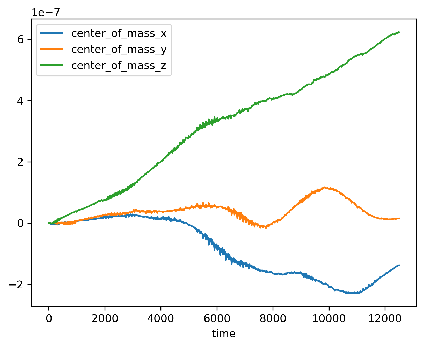
You can plot columns with the pandas plotting interface.
>>> ts.plot('time', ['center_of_mass_x', 'center_of_mass_y', 'center_of_mass_z'])
The previous code produces the following figure.
- 1
See https://pandas.pydata.org/ for more on pandas.