Analysis of SPH data
Subsnaps
When analyzing SPH data it can be useful to look at a subset of particles. For example, the simulation we have been working with has dust and gas. So far we have been plotting the total density. We may want to visualize the dust and gas separately.
To do this we make a SubSnap object. We can access these quantities
using the family() method. Given that there may be sub-types of
dust, using ‘dust’ returns a list by default. In this simulation there is only
one dust species. We can squeeze all the dust sub-types together using the
squeeze argument.
>>> gas = snap.family('gas')
>>> dust = snap.family('dust', squeeze=True)
You can access arrays on the SubSnap objects as for any
Snap object.
>>> gas['mass'].sum().to('solar_mass')
0.0010000000000000005 <Unit('solar_mass')>

>>> dust['mass'].sum().to('earth_mass')
3.326810503428664 <Unit('earth_mass')>
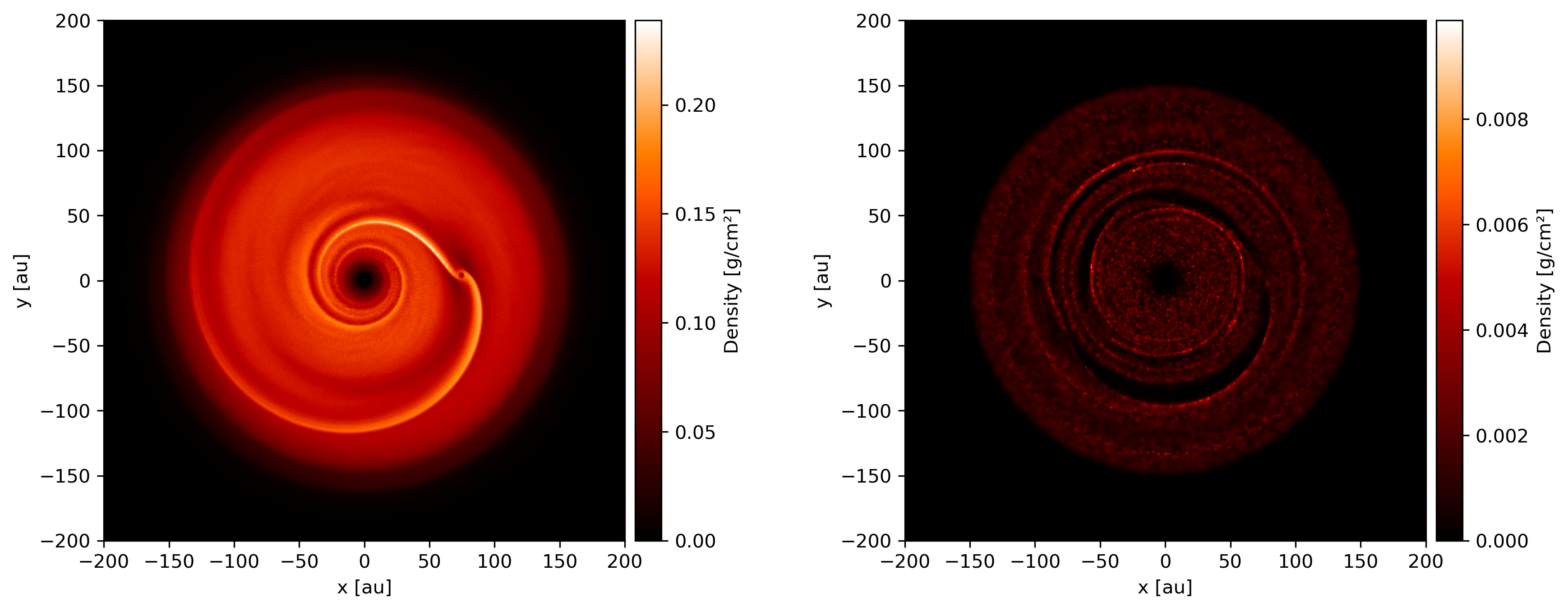
Let’s plot the gas and dust side-by-side.
>>> subsnaps = [gas, dust]
>>> extent = (-200, 200, -200, 200)

>>> fig, axs = plt.subplots(ncols=2, figsize=(14, 5))

>>> for subsnap, ax in zip(subsnaps, axs):
...     subsnap.image(quantity='density', extent=extent, cmap='gist_heat', ax=ax)
Derived arrays
Sometimes you need new arrays on the particles that are not available in the snapshot files. Many are available in Plonk already. The following code block lists the available raw Phantom arrays on the file.
>>> list(snap._file_pointer['particles'])
['divv', 'dt', 'dustfrac', 'h', 'itype', 'tstop', 'vxyz', 'xyz']
To see all available arrays on the Snap object:
>>> snap.available_arrays()
['angular_momentum',
 'angular_velocity',
 'azimuthal_angle',
 'density',
 'dust_to_gas_ratio',
 'id',
 'kinetic_energy',
 'mass',
 'momentum',
 'polar_angle',
 'position',
 'pressure',
 'radius_cylindrical',
 'radius_spherical',
 'smoothing_length',
 'sound_speed',
 'specific_angular_momentum',
 'specific_kinetic_energy',
 'stopping_time',
 'sub_type',
 'temperature',
 'timestep',
 'type',
 'velocity',
 'velocity_divergence',
 'velocity_radial_cylindrical',
 'velocity_radial_spherical']
This is a disc simulation. You can add quantities appropriate for discs with the
add_quantities() method.
>>> previous_arrays = snap.available_arrays()

>>> snap.add_quantities('disc')

# Additional available arrays
>>> set(snap.available_arrays()) - set(previous_arrays)
{'eccentricity',
 'inclination',
 'keplerian_frequency',
 'semi_major_axis',
 'stokes_number'}
You can create a new, derived array on the particles as follows.
>>> snap['rad'] = np.sqrt(snap['x'] ** 2 + snap['y'] ** 2)

>>> snap['rad']
array([8.28943225e+12, 2.00284678e+13, 1.79690392e+13, ...,
       1.81598604e+13, 1.38078875e+13, 2.08972008e+13]) <Unit('meter')>
Where, here, we have used the fact that Plonk knows that ‘x’ and ‘y’ refer to the x- and y-components of the position array.
Alternatively, you can define a function for a derived array. This makes use of
the decorator add_array().
>>> @snap.add_array()
... def radius(snap):
...     radius = np.hypot(snap['x'], snap['y'])
...     return radius

>>> snap['radius']
array([8.28943225e+12, 2.00284678e+13, 1.79690392e+13, ...,
       1.81598604e+13, 1.38078875e+13, 2.08972008e+13]) <Unit('meter')>
Units
Plonk uses Pint to set arrays to physical units.
>>> snap = plonk.load_snap(filename)

>>> snap['x']
array([-3.69505001e+12, -1.63052677e+13, -7.66283930e+12, ...,
        1.39571712e+13,  9.53716176e+12,  1.21421196e+12]) <Unit('meter')>
It is easy to convert quantities to different units as required.
>>> snap['x'].to('au')
array([ -24.6998837 , -108.99398271,  -51.22291689, ...,   93.29792694,
         63.75198868,    8.11650561]) <Unit('astronomical_unit')>
Profiles
Generating a profile is a convenient method to reduce the dimensionality of the full data set. For example, we may want to see how the surface density and aspect ratio of the disc vary with radius.
To do this we use the Profile class in the analysis module.
>>> snap = plonk.load_snap(filename)

>>> snap.add_quantities('disc')

>>> prof = plonk.load_profile(snap, cmin='10 au', cmax='200 au')

>>> prof
<plonk.Profile "disc_00030.h5">
To see what profiles are loaded and what are available use the
loaded_profiles() and available_profiles()
methods.
>>> prof.loaded_profiles()
['number', 'radius', 'size']

>>> prof.available_profiles()
['alpha_shakura_sunyaev',
 'angular_momentum_mag',
 'angular_momentum_phi',
 'angular_momentum_theta',
 'angular_momentum_x',
 'angular_momentum_y',
 'angular_momentum_z',
 'angular_velocity',
 'aspect_ratio',
 'azimuthal_angle',
 'density',
 'disc_viscosity',
 'dust_to_gas_ratio_001',
 'eccentricity',
 'epicyclic_frequency',
 'id',
 'inclination',
 'keplerian_frequency',
 'kinetic_energy',
 'mass',
 'midplane_stokes_number_001',
 'momentum_mag',
 'momentum_x',
 'momentum_y',
 'momentum_z',
 'number',
 'polar_angle',
 'position_mag',
 'position_x',
 'position_y',
 'position_z',
 'pressure',
 'radius',
 'radius_cylindrical',
 'radius_spherical',
 'scale_height',
 'semi_major_axis',
 'size',
 'smoothing_length',
 'sound_speed',
 'specific_angular_momentum_mag',
 'specific_angular_momentum_x',
 'specific_angular_momentum_y',
 'specific_angular_momentum_z',
 'specific_kinetic_energy',
 'stokes_number_001',
 'stopping_time_001',
 'sub_type',
 'surface_density',
 'temperature',
 'timestep',
 'toomre_q',
 'type',
 'velocity_divergence',
 'velocity_mag',
 'velocity_radial_cylindrical',
 'velocity_radial_spherical',
 'velocity_x',
 'velocity_y',
 'velocity_z']
To load a profile, simply call it.
>>> prof['scale_height']
array([7.97124951e+10, 9.84227660e+10, 1.18761140e+11, 1.37555034e+11,
       1.57492383e+11, 1.79386553e+11, 1.99666627e+11, 2.20898696e+11,
       2.46311866e+11, 2.63718852e+11, 2.91092881e+11, 3.11944125e+11,
       3.35101091e+11, 3.58479038e+11, 3.86137691e+11, 4.09731915e+11,
       4.34677739e+11, 4.61230912e+11, 4.87471032e+11, 5.07589421e+11,
       5.38769961e+11, 5.64068787e+11, 5.88487300e+11, 6.15197082e+11,
       6.35591229e+11, 6.75146081e+11, 6.94786320e+11, 7.32840731e+11,
       7.65750662e+11, 7.96047221e+11, 8.26764128e+11, 8.35658042e+11,
       8.57126522e+11, 8.99037935e+11, 9.26761324e+11, 9.45798955e+11,
       9.65997944e+11, 1.01555592e+12, 1.05554201e+12, 1.07641999e+12,
       1.10797835e+12, 1.13976869e+12, 1.17181502e+12, 1.20083661e+12,
       1.23779947e+12, 1.24785058e+12, 1.28800980e+12, 1.31290341e+12,
       1.33602542e+12, 1.34618607e+12, 1.36220344e+12, 1.39412340e+12,
       1.41778445e+12, 1.46713623e+12, 1.51140364e+12, 1.54496807e+12,
       1.58327631e+12, 1.60316504e+12, 1.63374960e+12, 1.64446331e+12,
       1.66063803e+12, 1.67890856e+12, 1.68505873e+12, 1.68507230e+12,
       1.71353612e+12, 1.71314330e+12, 1.75704484e+12, 1.79183025e+12,
       1.83696336e+12, 1.88823477e+12, 1.93080810e+12, 1.98301979e+12,
       2.05279086e+12, 2.11912539e+12, 2.14224572e+12, 2.21647741e+12,
       2.27153917e+12, 2.36605186e+12, 2.38922067e+12, 2.53901104e+12,
       2.61297334e+12, 2.64782574e+12, 2.73832897e+12, 3.04654121e+12,
       3.13575612e+12, 3.37636281e+12, 3.51482502e+12, 3.69591185e+12,
       3.88308614e+12, 3.83982313e+12, 4.00147149e+12, 4.37288049e+12,
       4.35330982e+12, 4.44686164e+12, 4.47133547e+12, 4.83307604e+12,
       4.63783507e+12, 4.95119779e+12, 5.17961431e+12, 5.29308491e+12]) <Unit('meter')>
You can convert the data in the Profile object to a pandas DataFrame
with the to_dataframe() method. This takes all loaded profiles
and puts them into the DataFrame with units indicated in brackets.
>>> profiles = [
...    'radius',
...    'angular_momentum_phi',
...    'angular_momentum_theta',
...    'surface_density',
...    'scale_height',
... ]

>>> df = prof.to_dataframe(columns=profiles)

>>> df
      radius [m]  angular_momentum_phi [rad]  angular_momentum_theta [rad]  surface_density [kg / m ** 2]  scale_height [m]
0   1.638097e+12                   -0.019731                      0.049709                       0.486007      7.971250e+10
1   1.922333e+12                    1.914841                      0.053297                       0.630953      9.842277e+10
2   2.206569e+12                    1.293811                      0.055986                       0.808415      1.187611e+11
3   2.490805e+12                   -2.958286                      0.057931                       0.956107      1.375550e+11
4   2.775041e+12                   -1.947547                      0.059679                       1.095939      1.574924e+11
..           ...                         ...                           ...                            ...               ...
95  2.864051e+13                    3.045660                      0.168944                       0.013883      4.833076e+12
96  2.892475e+13                   -0.054956                      0.161673                       0.013246      4.637835e+12
97  2.920898e+13                   -0.217485                      0.169546                       0.011058      4.951198e+12
98  2.949322e+13                   -1.305261                      0.175302                       0.011367      5.179614e+12
99  2.977746e+13                    2.642077                      0.176867                       0.010660      5.293085e+12

[100 rows x 5 columns]
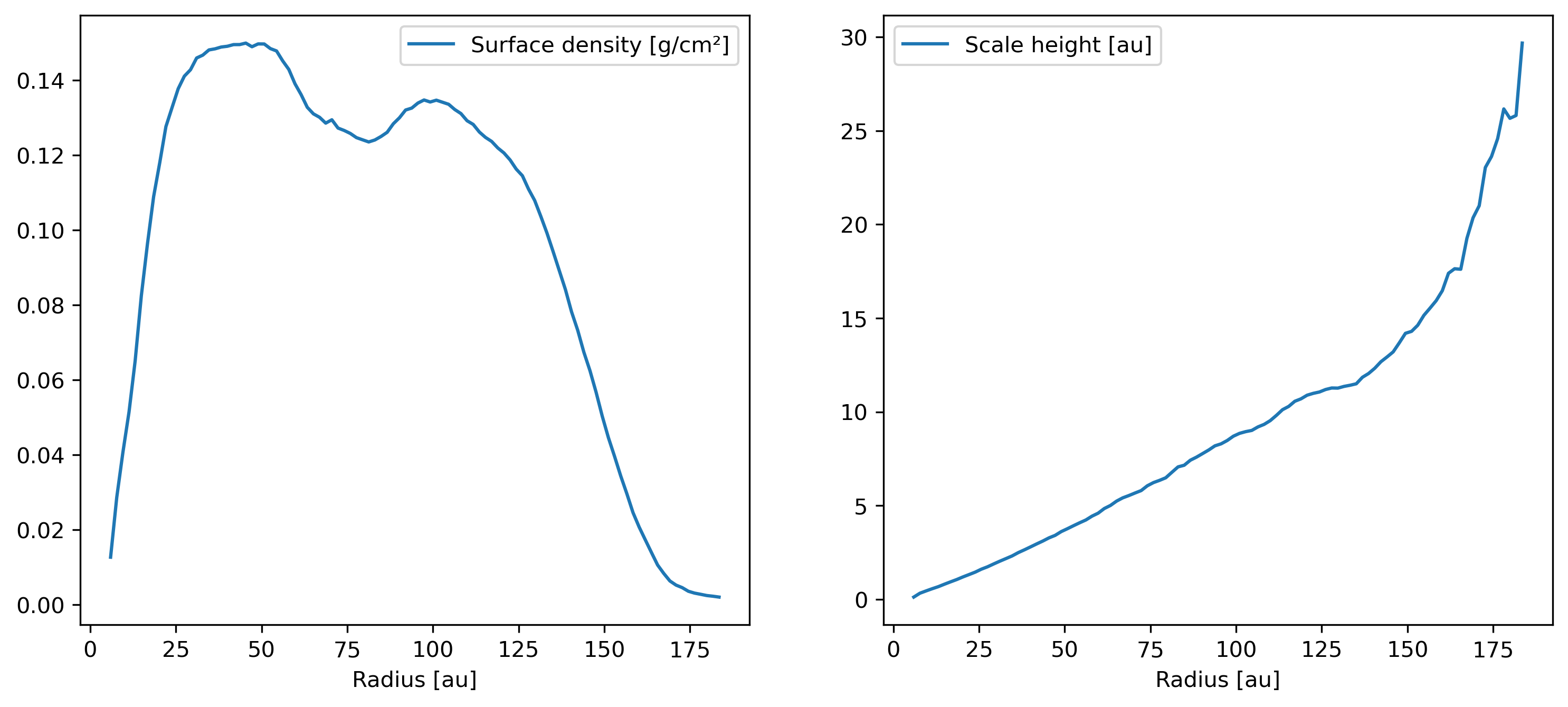
We can also plot the profiles.
>>> prof.set_units(position='au', scale_height='au', surface_density='g/cm^2')

>>> fig, axs = plt.subplots(ncols=2, figsize=(12, 5))

>>> prof.plot('radius', 'surface_density', ax=axs[0])

>>> prof.plot('radius', 'scale_height', ax=axs[1])